- Artificial Neural Network Tutorial
- Artificial Neural Network - Home
- Basic Concepts
- Building Blocks
- Learning & Adaptation
- Supervised Learning
- Unsupervised Learning
- Learning Vector Quantization
- Adaptive Resonance Theory
- Kohonen Self-Organizing Feature Maps
- Associate Memory Network
- Hopfield Networks
- Boltzmann Machine
- Brain-State-in-a-Box Network
- Optimization Using Hopfield Network
- Other Optimization Techniques
- Genetic Algorithm
- Applications of Neural Networks
- Artificial Neural Network Resources
- Quick Guide
- Useful Resources
- Discussion
Adaptive Resonance Theory
This network was developed by Stephen Grossberg and Gail Carpenter in 1987. It is based on competition and uses unsupervised learning model. Adaptive Resonance Theory (ART) networks, as the name suggests, is always open to new learning (adaptive) without losing the old patterns (resonance). Basically, ART network is a vector classifier which accepts an input vector and classifies it into one of the categories depending upon which of the stored pattern it resembles the most.
Operating Principal
The main operation of ART classification can be divided into the following phases −
Recognition phase − The input vector is compared with the classification presented at every node in the output layer. The output of the neuron becomes “1” if it best matches with the classification applied, otherwise it becomes “0”.
Comparison phase − In this phase, a comparison of the input vector to the comparison layer vector is done. The condition for reset is that the degree of similarity would be less than vigilance parameter.
Search phase − In this phase, the network will search for reset as well as the match done in the above phases. Hence, if there would be no reset and the match is quite good, then the classification is over. Otherwise, the process would be repeated and the other stored pattern must be sent to find the correct match.
ART1
It is a type of ART, which is designed to cluster binary vectors. We can understand about this with the architecture of it.
Architecture of ART1
It consists of the following two units −
Computational Unit − It is made up of the following −
Input unit (F1 layer) − It further has the following two portions −
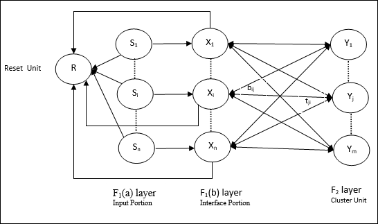
F1(a) layer (Input portion) − In ART1, there would be no processing in this portion rather than having the input vectors only. It is connected to F1(b) layer (interface portion).
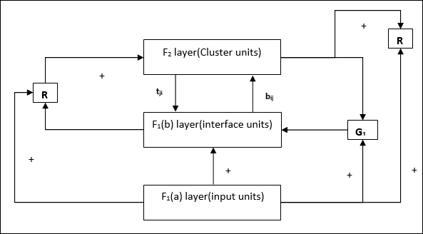
F1(b) layer (Interface portion) − This portion combines the signal from the input portion with that of F2 layer. F1(b) layer is connected to F2 layer through bottom up weights bij and F2 layer is connected to F1(b) layer through top down weights tji.
Cluster Unit (F2 layer) − This is a competitive layer. The unit having the largest net input is selected to learn the input pattern. The activation of all other cluster unit are set to 0.
Reset Mechanism − The work of this mechanism is based upon the similarity between the top-down weight and the input vector. Now, if the degree of this similarity is less than the vigilance parameter, then the cluster is not allowed to learn the pattern and a rest would happen.
Supplement Unit − Actually the issue with Reset mechanism is that the layer F2 must have to be inhibited under certain conditions and must also be available when some learning happens. That is why two supplemental units namely, G1 and G2 is added along with reset unit, R. They are called gain control units. These units receive and send signals to the other units present in the network. ‘+’ indicates an excitatory signal, while ‘−’ indicates an inhibitory signal.


Parameters Used
Following parameters are used −
n − Number of components in the input vector
m − Maximum number of clusters that can be formed
bij − Weight from F1(b) to F2 layer, i.e. bottom-up weights
tji − Weight from F2 to F1(b) layer, i.e. top-down weights
ρ − Vigilance parameter
||x|| − Norm of vector x
Algorithm
Step 1 − Initialize the learning rate, the vigilance parameter, and the weights as follows −
$$\alpha\:>\:1\:\:and\:\:0\:<\rho\:\leq\:1$$
$$0\:<\:b_{ij}(0)\:<\:\frac{\alpha}{\alpha\:-\:1\:+\:n}\:\:and\:\:t_{ij}(0)\:=\:1$$
Step 2 − Continue step 3-9, when the stopping condition is not true.
Step 3 − Continue step 4-6 for every training input.
Step 4 − Set activations of all F1(a) and F1 units as follows
F2 = 0 and F1(a) = input vectors
Step 5 − Input signal from F1(a) to F1(b) layer must be sent like
$$s_{i}\:=\:x_{i}$$
Step 6 − For every inhibited F2 node
$y_{j}\:=\:\sum_i b_{ij}x_{i}$ the condition is yj ≠ -1
Step 7 − Perform step 8-10, when the reset is true.
Step 8 − Find J for yJ ≥ yj for all nodes j
Step 9 − Again calculate the activation on F1(b) as follows
$$x_{i}\:=\:sitJi$$
Step 10 − Now, after calculating the norm of vector x and vector s, we need to check the reset condition as follows −
If ||x||/ ||s|| < vigilance parameter ρ,theninhibit node J and go to step 7
Else If ||x||/ ||s|| ≥ vigilance parameter ρ, then proceed further.
Step 11 − Weight updating for node J can be done as follows −
$$b_{ij}(new)\:=\:\frac{\alpha x_{i}}{\alpha\:-\:1\:+\:||x||}$$
$$t_{ij}(new)\:=\:x_{i}$$
Step 12 − The stopping condition for algorithm must be checked and it may be as follows −
- Do not have any change in weight.
- Reset is not performed for units.
- Maximum number of epochs reached.
To Continue Learning Please Login